Scaling a Subset of Input Data in NetCDF Format
Reference: For general python handling of nc files using Xarray: http://xarray.pydata.org/en/stable/index.html
I was working on a set of input data of Ocean DMS concentration. I suspected the reported values over the Southern Ocean (vaguely defined as ocean south to 30ºS) were a bit high. I wanted to reduce those values by 50% to see if my model would match observations better. 🌊
Surprisingly, I couldn’t find a quick way to do it. Here I present a workaround. (Please let me know if you have a smarter way! 💡)
import wget                        # for downloading data via URL links
import xarray as xr                   # the major tool to work with NetCDF data!
from matplotlib import pyplot as plt  # for plotting
Open the monthly Ocean DMS nc file
The marine DMS data used in this example can be downloaded from the Dalhousie University server. Or, we can download it from Python.
wget.download('http://rain.ucis.dal.ca/ctm/HEMCO/DMS/v2015-07/DMS_lana.geos.1x1.nc')
'DMS_lana.geos.1x1.nc'
We will use the function xr.open_dataset from the xarray package.
ds = xr.open_dataset('DMS_lana.geos.1x1.nc')

ds # display the dataset
<xarray.Dataset>
Dimensions: (lat: 181, lon: 360, time: 12)
Coordinates:
- lon (lon) float32 -180.0 -179.0 -178.0 -177.0 … 177.0 178.0 179.0
- lat (lat) float32 -89.75 -89.0 -88.0 -87.0 … 87.0 88.0 89.0 89.75
- time (time) datetime64[ns] 1985-01-01 1985-02-01 … 1985-12-01
Data variables:
DMS_OCEAN (time, lat, lon) float32 …
Attributes:
CDI: Climate Data Interface version 1.6.4 (http://code.zmaw.de/p…
Conventions: COARDS
history: Mon Jul 20 16:29:35 2015: ncatted -O -a units,DMS_OCEAN,o,c…
Title: COARDS/netCDF file created by BPCH2COARDS (GAMAP v2-17+)
Format: NetCDF-3
Model: GEOS5_47L
Delta_Lon: 1.0
Delta_Lat: 1.0
NLayers: 47
Start_Date: 19850101
Start_Time: 0
End_Date: 19850201
End_Time: 0
Delta_Time: 744
CDO: Climate Data Operators version 1.6.4 (http://code.zmaw.de/p…xarray.Dataset
- lat: 181
- lon: 360
- time: 12
- lon(lon)float32-180.0 -179.0 … 178.0 179.0
- standard_name :
- longitude
- long_name :
- Longitude
- units :
- degrees_east
- axis :
- X
array([-180., -179., -178., …, 177., 178., 179.], dtype=float32)
- lat(lat)float32-89.75 -89.0 -88.0 … 89.0 89.75
- standard_name :
- latitude
- long_name :
- Latitude
- units :
- degrees_north
- axis :
- Y
array([-89.75, -89. , -88. , -87. , -86. , -85. , -84. , -83. , -82. ,
-81. , -80. , -79. , -78. , -77. , -76. , -75. , -74. , -73. ,
-72. , -71. , -70. , -69. , -68. , -67. , -66. , -65. , -64. ,
-63. , -62. , -61. , -60. , -59. , -58. , -57. , -56. , -55. ,
-54. , -53. , -52. , -51. , -50. , -49. , -48. , -47. , -46. ,
-45. , -44. , -43. , -42. , -41. , -40. , -39. , -38. , -37. ,
-36. , -35. , -34. , -33. , -32. , -31. , -30. , -29. , -28. ,
-27. , -26. , -25. , -24. , -23. , -22. , -21. , -20. , -19. ,
-18. , -17. , -16. , -15. , -14. , -13. , -12. , -11. , -10. ,
-9. , -8. , -7. , -6. , -5. , -4. , -3. , -2. , -1. ,
0. , 1. , 2. , 3. , 4. , 5. , 6. , 7. , 8. ,
9. , 10. , 11. , 12. , 13. , 14. , 15. , 16. , 17. ,
18. , 19. , 20. , 21. , 22. , 23. , 24. , 25. , 26. ,
27. , 28. , 29. , 30. , 31. , 32. , 33. , 34. , 35. ,
36. , 37. , 38. , 39. , 40. , 41. , 42. , 43. , 44. ,
45. , 46. , 47. , 48. , 49. , 50. , 51. , 52. , 53. ,
54. , 55. , 56. , 57. , 58. , 59. , 60. , 61. , 62. ,
63. , 64. , 65. , 66. , 67. , 68. , 69. , 70. , 71. ,
72. , 73. , 74. , 75. , 76. , 77. , 78. , 79. , 80. ,
81. , 82. , 83. , 84. , 85. , 86. , 87. , 88. , 89. ,
89.75], dtype=float32)
- time(time)datetime64[ns]1985-01-01 … 1985-12-01
- standard_name :
- time
- long_name :
- Time
array(['1985-01-01T00:00:00.000000000', '1985-02-01T00:00:00.000000000',
'1985-03-01T00:00:00.000000000', '1985-04-01T00:00:00.000000000',
'1985-05-01T00:00:00.000000000', '1985-06-01T00:00:00.000000000',
'1985-07-01T00:00:00.000000000', '1985-08-01T00:00:00.000000000',
'1985-09-01T00:00:00.000000000', '1985-10-01T00:00:00.000000000',
'1985-11-01T00:00:00.000000000', '1985-12-01T00:00:00.000000000'],
dtype='datetime64[ns]')
- DMS_OCEAN(time, lat, lon)float32…
- long_name :
- Ocean DMS concentration
- units :
- kg/m3
[781920 values with dtype=float32]
- CDI :
- Climate Data Interface version 1.6.4 (http://code.zmaw.de/projects/cdi)
- Conventions :
- COARDS
- history :
- Mon Jul 20 16:29:35 2015: ncatted -O -a units,DMS_OCEAN,o,c,kg/m3 tmp3.nc Mon Jul 20 16:29:34 2015: cdo mulc,6.213e-8 tmp2.nc tmp3.nc Mon Jul 20 16:29:34 2015: cdo chname,BIOGSRCE__DMSOCN,DMS_OCEAN tmp.nc tmp2.nc Mon Jul 20 16:29:34 2015: cdo mergetime tmp.1985*.nc tmp.nc
- Title :
- COARDS/netCDF file created by BPCH2COARDS (GAMAP v2-17+)
- Format :
- NetCDF-3
- Model :
- GEOS5_47L
- Delta_Lon :
- 1.0
- Delta_Lat :
- 1.0
- NLayers :
- 47
- Start_Date :
- 19850101
- Start_Time :
- 0
- End_Date :
- 19850201
- End_Time :
- 0
- Delta_Time :
- 744
- CDO :
- Climate Data Operators version 1.6.4 (http://code.zmaw.de/projects/cdo)
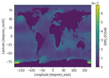
We can also visualize annual mean of the data for a quick check:
ds['DMS_OCEAN'].mean(dim=['time']).plot()
<matplotlib.collections.QuadMesh at 0x7fd61bbd01f0>
Scaling down the Southern Ocean DMS
As mentioned, we want to scale down the ocean DMS below 30ºS.
# Step 1: make two copies of the data set, one for grid cells with lat > 30ºS, one for <30ºS

dms_above30S = ds['DMS_OCEAN'].sel(lat=slice(-30,90))

dms_below30S = ds['DMS_OCEAN'].sel(lat=slice(-90,-30-1e-9)) # we add a small value here to avoid the grid cells with lat = 30ºS to appear in both data sets.

# Step 2: reduce the DMS in the dataset of interest by 50%

dms_below30S = dms_below30S * 0.5

# Step 3: merge the untouched and scaled data
ds_partly_scaled = xr.merge([dms_below30S, dms_above30S], compat="no_conflicts")
To ensure our exercise is correct, let’s make some plots to compare the DMS concentrations in ds_partly_scaled and the original dataset, ds.
(ds_partly_scaled['DMS_OCEAN'] / ds['DMS_OCEAN']).plot(col='time', col_wrap=3)
<xarray.plot.facetgrid.FacetGrid at 0x7fd61bd3ba00>
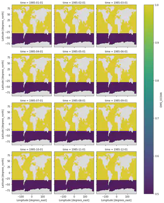
Yellow = 1 (untouched); Purple = 0.5(scaled). Mission accomplished?
ds_partly_scaled # missing attributes from the original dataset.
<xarray.Dataset>
Dimensions: (lat: 181, lon: 360, time: 12)
Coordinates:
-
lat (lat) float64 -89.75 -89.0 -88.0 -87.0 … 87.0 88.0 89.0 89.75
-
lon (lon) float32 -180.0 -179.0 -178.0 -177.0 … 177.0 178.0 179.0
-
time (time) datetime64[ns] 1985-01-01 1985-02-01 … 1985-12-01 Data variables: DMS_OCEAN (time, lat, lon) float32 0.0 0.0 … 1.4103641e-07 1.4103641e-07
xarray.Dataset- lat: 181
- lon: 360
- time: 12
- lat(lat)float64-89.75 -89.0 -88.0 … 89.0 89.75
- standard_name :
- latitude
- long_name :
- Latitude
- units :
- degrees_north
- axis :
- Y
array([-89.75, -89. , -88. , -87. , -86. , -85. , -84. , -83. , -82. ,
-81. , -80. , -79. , -78. , -77. , -76. , -75. , -74. , -73. ,
-72. , -71. , -70. , -69. , -68. , -67. , -66. , -65. , -64. ,
-63. , -62. , -61. , -60. , -59. , -58. , -57. , -56. , -55. ,
-54. , -53. , -52. , -51. , -50. , -49. , -48. , -47. , -46. ,
-45. , -44. , -43. , -42. , -41. , -40. , -39. , -38. , -37. ,
-36. , -35. , -34. , -33. , -32. , -31. , -30. , -29. , -28. ,
-27. , -26. , -25. , -24. , -23. , -22. , -21. , -20. , -19. ,
-18. , -17. , -16. , -15. , -14. , -13. , -12. , -11. , -10. ,
-9. , -8. , -7. , -6. , -5. , -4. , -3. , -2. , -1. ,
0. , 1. , 2. , 3. , 4. , 5. , 6. , 7. , 8. ,
9. , 10. , 11. , 12. , 13. , 14. , 15. , 16. , 17. ,
18. , 19. , 20. , 21. , 22. , 23. , 24. , 25. , 26. ,
27. , 28. , 29. , 30. , 31. , 32. , 33. , 34. , 35. ,
36. , 37. , 38. , 39. , 40. , 41. , 42. , 43. , 44. ,
45. , 46. , 47. , 48. , 49. , 50. , 51. , 52. , 53. ,
54. , 55. , 56. , 57. , 58. , 59. , 60. , 61. , 62. ,
63. , 64. , 65. , 66. , 67. , 68. , 69. , 70. , 71. ,
72. , 73. , 74. , 75. , 76. , 77. , 78. , 79. , 80. ,
81. , 82. , 83. , 84. , 85. , 86. , 87. , 88. , 89. ,
89.75])
- lon(lon)float32-180.0 -179.0 … 178.0 179.0
- standard_name :
- longitude
- long_name :
- Longitude
- units :
- degrees_east
- axis :
- X
array([-180., -179., -178., …, 177., 178., 179.], dtype=float32)
- time(time)datetime64[ns]1985-01-01 … 1985-12-01
- standard_name :
- time
- long_name :
- Time
array(['1985-01-01T00:00:00.000000000', '1985-02-01T00:00:00.000000000',
'1985-03-01T00:00:00.000000000', '1985-04-01T00:00:00.000000000',
'1985-05-01T00:00:00.000000000', '1985-06-01T00:00:00.000000000',
'1985-07-01T00:00:00.000000000', '1985-08-01T00:00:00.000000000',
'1985-09-01T00:00:00.000000000', '1985-10-01T00:00:00.000000000',
'1985-11-01T00:00:00.000000000', '1985-12-01T00:00:00.000000000'],
dtype='datetime64[ns]')
- DMS_OCEAN(time, lat, lon)float320.0 0.0 … 1.4103641e-07
array([[[0.0000000e+00, 0.0000000e+00, 0.0000000e+00, …, 0.0000000e+00, 0.0000000e+00, 0.0000000e+00], [0.0000000e+00, 0.0000000e+00, 0.0000000e+00, …, 0.0000000e+00, 0.0000000e+00, 0.0000000e+00], [0.0000000e+00, 0.0000000e+00, 0.0000000e+00, …, 0.0000000e+00, 0.0000000e+00, 0.0000000e+00], …, [1.0823291e-07, 1.0823291e-07, 1.0823291e-07, …, 1.0823291e-07, 1.0823291e-07, 1.0823291e-07], [1.0823292e-07, 1.0823292e-07, 1.0823292e-07, …, 1.0823292e-07, 1.0823292e-07, 1.0823292e-07], [2.1647536e-07, 2.1647536e-07, 2.1647536e-07, …, 2.1647536e-07, 2.1647536e-07, 2.1647536e-07]],
[[0.0000000e+00, 0.0000000e+00, 0.0000000e+00, ..., 0.0000000e+00, 0.0000000e+00, 0.0000000e+00], [0.0000000e+00, 0.0000000e+00, 0.0000000e+00, ..., 0.0000000e+00, 0.0000000e+00, 0.0000000e+00], [0.0000000e+00, 0.0000000e+00, 0.0000000e+00, ..., 0.0000000e+00, 0.0000000e+00, 0.0000000e+00],… [4.1650505e-08, 4.1650505e-08, 4.1650505e-08, …, 4.1650505e-08, 4.1650505e-08, 4.1650505e-08], [4.1650505e-08, 4.1650505e-08, 4.1650505e-08, …, 4.1650505e-08, 4.1650505e-08, 4.1650505e-08], [8.3304677e-08, 8.3304677e-08, 8.3304677e-08, …, 8.3304677e-08, 8.3304677e-08, 8.3304677e-08]],
[[0.0000000e+00, 0.0000000e+00, 0.0000000e+00, ..., 0.0000000e+00, 0.0000000e+00, 0.0000000e+00], [0.0000000e+00, 0.0000000e+00, 0.0000000e+00, ..., 0.0000000e+00, 0.0000000e+00, 0.0000000e+00], [0.0000000e+00, 0.0000000e+00, 0.0000000e+00, ..., 0.0000000e+00, 0.0000000e+00, 0.0000000e+00], ..., [7.0515100e-08, 7.0515100e-08, 7.0515100e-08, ..., 7.0515100e-08, 7.0515100e-08, 7.0515100e-08], [7.0515107e-08, 7.0515107e-08, 7.0515107e-08, ..., 7.0515107e-08, 7.0515107e-08, 7.0515107e-08], [1.4103641e-07, 1.4103641e-07, 1.4103641e-07, ..., 1.4103641e-07, 1.4103641e-07, 1.4103641e-07]]], dtype=float32)</pre></div></li></ul></div></li><li class='xr-section-item'><input id='section-7d38814c-2b4b-4a64-b9af-a8732a4af998' class='xr-section-summary-in' type='checkbox' disabled ><label for='section-7d38814c-2b4b-4a64-b9af-a8732a4af998' class='xr-section-summary' title='Expand/collapse section'>Attributes: <span>(0)</span></label><div class='xr-section-inline-details'></div><div class='xr-section-details'><dl class='xr-attrs'></dl></div></li></ul></div></div>Preserving metadata from the original nc file
Not yet! Now the new merged data set is missing the Attributes of the original.
To fix this, we need to make a xarray copy of the original to preserve the original information, but with the new scaled values.
ds_new = ds.copy(data=ds_partly_scaled) ds_new # now with the Attributes<xarray.Dataset> Dimensions: (lat: 181, lon: 360, time: 12) Coordinates:
-
lon (lon) float32 -180.0 -179.0 -178.0 -177.0 … 177.0 178.0 179.0
-
lat (lat) float64 -89.75 -89.0 -88.0 -87.0 … 87.0 88.0 89.0 89.75
-
time (time) datetime64[ns] 1985-01-01 1985-02-01 … 1985-12-01 Data variables: DMS_OCEAN (time, lat, lon) float32 0.0 0.0 … 1.4103641e-07 1.4103641e-07 Attributes: CDI: Climate Data Interface version 1.6.4 (http://code.zmaw.de/p… Conventions: COARDS history: Mon Jul 20 16:29:35 2015: ncatted -O -a units,DMS_OCEAN,o,c… Title: COARDS/netCDF file created by BPCH2COARDS (GAMAP v2-17+) Format: NetCDF-3 Model: GEOS5_47L Delta_Lon: 1.0 Delta_Lat: 1.0 NLayers: 47 Start_Date: 19850101 Start_Time: 0 End_Date: 19850201 End_Time: 0 Delta_Time: 744 CDO: Climate Data Operators version 1.6.4 (http://code.zmaw.de/p…
xarray.Dataset- lat: 181
- lon: 360
- time: 12
- lon(lon)float32-180.0 -179.0 … 178.0 179.0
- standard_name :
- longitude
- long_name :
- Longitude
- units :
- degrees_east
- axis :
- X
array([-180., -179., -178., …, 177., 178., 179.], dtype=float32)
- lat(lat)float64-89.75 -89.0 -88.0 … 89.0 89.75
- standard_name :
- latitude
- long_name :
- Latitude
- units :
- degrees_north
- axis :
- Y
array([-89.75, -89. , -88. , -87. , -86. , -85. , -84. , -83. , -82. , -81. , -80. , -79. , -78. , -77. , -76. , -75. , -74. , -73. , -72. , -71. , -70. , -69. , -68. , -67. , -66. , -65. , -64. , -63. , -62. , -61. , -60. , -59. , -58. , -57. , -56. , -55. , -54. , -53. , -52. , -51. , -50. , -49. , -48. , -47. , -46. , -45. , -44. , -43. , -42. , -41. , -40. , -39. , -38. , -37. , -36. , -35. , -34. , -33. , -32. , -31. , -30. , -29. , -28. , -27. , -26. , -25. , -24. , -23. , -22. , -21. , -20. , -19. , -18. , -17. , -16. , -15. , -14. , -13. , -12. , -11. , -10. , -9. , -8. , -7. , -6. , -5. , -4. , -3. , -2. , -1. , 0. , 1. , 2. , 3. , 4. , 5. , 6. , 7. , 8. , 9. , 10. , 11. , 12. , 13. , 14. , 15. , 16. , 17. , 18. , 19. , 20. , 21. , 22. , 23. , 24. , 25. , 26. , 27. , 28. , 29. , 30. , 31. , 32. , 33. , 34. , 35. , 36. , 37. , 38. , 39. , 40. , 41. , 42. , 43. , 44. , 45. , 46. , 47. , 48. , 49. , 50. , 51. , 52. , 53. , 54. , 55. , 56. , 57. , 58. , 59. , 60. , 61. , 62. , 63. , 64. , 65. , 66. , 67. , 68. , 69. , 70. , 71. , 72. , 73. , 74. , 75. , 76. , 77. , 78. , 79. , 80. , 81. , 82. , 83. , 84. , 85. , 86. , 87. , 88. , 89. , 89.75])
- time(time)datetime64[ns]1985-01-01 … 1985-12-01
- standard_name :
- time
- long_name :
- Time
array(['1985-01-01T00:00:00.000000000', '1985-02-01T00:00:00.000000000', '1985-03-01T00:00:00.000000000', '1985-04-01T00:00:00.000000000', '1985-05-01T00:00:00.000000000', '1985-06-01T00:00:00.000000000', '1985-07-01T00:00:00.000000000', '1985-08-01T00:00:00.000000000', '1985-09-01T00:00:00.000000000', '1985-10-01T00:00:00.000000000', '1985-11-01T00:00:00.000000000', '1985-12-01T00:00:00.000000000'], dtype='datetime64[ns]')
- DMS_OCEAN(time, lat, lon)float320.0 0.0 … 1.4103641e-07
- long_name :
- Ocean DMS concentration
- units :
- kg/m3
array([[[0.0000000e+00, 0.0000000e+00, 0.0000000e+00, …, 0.0000000e+00, 0.0000000e+00, 0.0000000e+00], [0.0000000e+00, 0.0000000e+00, 0.0000000e+00, …, 0.0000000e+00, 0.0000000e+00, 0.0000000e+00], [0.0000000e+00, 0.0000000e+00, 0.0000000e+00, …, 0.0000000e+00, 0.0000000e+00, 0.0000000e+00], …, [1.0823291e-07, 1.0823291e-07, 1.0823291e-07, …, 1.0823291e-07, 1.0823291e-07, 1.0823291e-07], [1.0823292e-07, 1.0823292e-07, 1.0823292e-07, …, 1.0823292e-07, 1.0823292e-07, 1.0823292e-07], [2.1647536e-07, 2.1647536e-07, 2.1647536e-07, …, 2.1647536e-07, 2.1647536e-07, 2.1647536e-07]],
[[0.0000000e+00, 0.0000000e+00, 0.0000000e+00, ..., 0.0000000e+00, 0.0000000e+00, 0.0000000e+00], [0.0000000e+00, 0.0000000e+00, 0.0000000e+00, ..., 0.0000000e+00, 0.0000000e+00, 0.0000000e+00], [0.0000000e+00, 0.0000000e+00, 0.0000000e+00, ..., 0.0000000e+00, 0.0000000e+00, 0.0000000e+00],… [4.1650505e-08, 4.1650505e-08, 4.1650505e-08, …, 4.1650505e-08, 4.1650505e-08, 4.1650505e-08], [4.1650505e-08, 4.1650505e-08, 4.1650505e-08, …, 4.1650505e-08, 4.1650505e-08, 4.1650505e-08], [8.3304677e-08, 8.3304677e-08, 8.3304677e-08, …, 8.3304677e-08, 8.3304677e-08, 8.3304677e-08]],
[[0.0000000e+00, 0.0000000e+00, 0.0000000e+00, ..., 0.0000000e+00, 0.0000000e+00, 0.0000000e+00], [0.0000000e+00, 0.0000000e+00, 0.0000000e+00, ..., 0.0000000e+00, 0.0000000e+00, 0.0000000e+00], [0.0000000e+00, 0.0000000e+00, 0.0000000e+00, ..., 0.0000000e+00, 0.0000000e+00, 0.0000000e+00], ..., [7.0515100e-08, 7.0515100e-08, 7.0515100e-08, ..., 7.0515100e-08, 7.0515100e-08, 7.0515100e-08], [7.0515107e-08, 7.0515107e-08, 7.0515107e-08, ..., 7.0515107e-08, 7.0515107e-08, 7.0515107e-08], [1.4103641e-07, 1.4103641e-07, 1.4103641e-07, ..., 1.4103641e-07, 1.4103641e-07, 1.4103641e-07]]], dtype=float32)</pre></div></li></ul></div></li><li class='xr-section-item'><input id='section-a5022503-e091-4ad2-a439-4f7e4b523a52' class='xr-section-summary-in' type='checkbox' ><label for='section-a5022503-e091-4ad2-a439-4f7e4b523a52' class='xr-section-summary' >Attributes: <span>(15)</span></label><div class='xr-section-inline-details'></div><div class='xr-section-details'><dl class='xr-attrs'><dt><span>CDI :</span></dt><dd>Climate Data Interface version 1.6.4 (http://code.zmaw.de/projects/cdi)</dd><dt><span>Conventions :</span></dt><dd>COARDS</dd><dt><span>history :</span></dt><dd>Mon Jul 20 16:29:35 2015: ncatted -O -a units,DMS_OCEAN,o,c,kg/m3 tmp3.ncMon Jul 20 16:29:34 2015: cdo mulc,6.213e-8 tmp2.nc tmp3.nc Mon Jul 20 16:29:34 2015: cdo chname,BIOGSRCE__DMSOCN,DMS_OCEAN tmp.nc tmp2.nc Mon Jul 20 16:29:34 2015: cdo mergetime tmp.1985*.nc tmp.nc
- Title :
- COARDS/netCDF file created by BPCH2COARDS (GAMAP v2-17+)
- Format :
- NetCDF-3
- Model :
- GEOS5_47L
- Delta_Lon :
- 1.0
- Delta_Lat :
- 1.0
- NLayers :
- 47
- Start_Date :
- 19850101
- Start_Time :
- 0
- End_Date :
- 19850201
- End_Time :
- 0
- Delta_Time :
- 744
- CDO :
- Climate Data Operators version 1.6.4 (http://code.zmaw.de/projects/cdo)
Finally, save the scaled DMS in a new file
And, it’s one-line easy.
ds_new.to_netcdf('DMS_lana.geos.1x1.SouthernHalved.nc') # always good to have a descriptive nameAgain, I know that it’s likely not the best way. Please let me know if you have a smarter way. I am always open to learn!
-